de Brogli wavelength

• Interference, diffraction and polarization establishes the wave nature of light and can be explained on the basis of wave theory
• photoelectric effect and compton effect are explained on the basis of quantum theory of light which establishes that quanta behaves like corpescules.
• Louis de Brogli proposed that idea of dual nature i.e., wave particle duality should be extanded to all micro particlesi.e., wave and corpescular nature should be associated with each particle.
• According to him material particles might have dual nature same as that of light.
• He suggested that moving particle whatever is its nature , has wave properties associated with it.
• Wavelength λ associated with any particle of momentum p is given by
  λ=h/p=h/mv
  where h is the Plank's constant.
• From Plank's theory of radiation , energy of photon is given by
  E=hν = hc/λ
  therefore λ=hc/E
  From special theory of relativity
  E=mc²
  mass of photon is m=hν/c²
  momentum of photon is
  mc=p=hν/c = h/λ
  therefore p=h/λ
  or, λ=h/p
• Thus what is true for energy packet (photon) is also true for material particle. Thus, for particle of mass m moving with velocity v , we have p=mv and de Brogli wavelength associated with it is
  λ=h/mv
  where m is the relativistic mass of the particle
• If m or v is large the de Brogli wavelength associated with a material particle would be small.
• The de Brogli wave associated with a material particle or photon of any charge associated with it can also be calculated. Thus we know that
  K=mv²/2
  therefore mv=√(2mK)
  λ=h/√(2mK)
• If a charged particle carrying a charge q is accelerated through a potential difference V volts, then kinetic energy K=qV
  Therefore be Brogli wavelength of charge particle for charge q and accelerated through a potential difference of V volts is given by
  λ=h/√(2mqV)

One Dimensional Oscillator (small oscillations)

• Consider a system with one degree of freedom and one generalized co-ordinate q. For small displacement from the equilibrium we can expand potential energy function using taylor series expansion about the equilibrium and we will only consider the lowest order terms. So expanding PE function V(q) we have
  
  
  
  
  
  
  where derivativesare evaluated at the equilibrium position q=q₀ and at equlilbrium (∂V/∂q)₀ = 0
• V(q₀) is potential energy at equilibrium and can be taken as zero, if the origin of potential energy is shifted to be at minimum equilibrium value.
  This implies that
  
  
  
  
  
  
  
  
  putting second derivative term in bracket equal to k and shifting origin to q₀=0 we have
  V(q)=kq²/2
  and k is the positive parameter at the position of stable equilibrium.
• If generalized co-ordinates does not involve time explicitely , the K.E. is then homogeneous quadratic function of generalized velocities, or,.
  
  

where coefficent m(q) , is in general function of q co-ordinate and may also be expanded in taylor series about the equilibrium position as we have done for potential energy function and first derivative of q is quadratic in this equation and the lowest lowest nonvanishing approximation to T is obtained by retaining only the firt term in the Taylor series expansion of m(q) which is m(0). Thus Lagrangian for small oscillations of one dimensional oscillator is

and equation of motion is

Stable and unstable equilibrium

First consider the figures given below

• Above are the plots of potential energy as a function of x , for a particle executing bound and unbound motion.
• At x₀=0 slope of potential energy curve dV/dx is zero. this implies that F = 0 i.e.,
          F = -dV/dx = 0                 (1)
  and a point particle placed at such a point with zero velocity will continue to remain at rest.
• At point x₀ in figugure (a) at which potential energy has a minimum , if the particle is displaced then the force F = -dV/dx will tend to return to it and it will oscillate about the equilibrium point, performing bound motion. These points are called points of stable equilibrium.
• If the particle is displaced slightly from the equilibrium x₀ in figure (b) , then it will be acted upon by the force
        F(x) = -(-dV/dx) = dV/dx          (2)
  which will tend to push away the particle from equilibrium point , when released. Such points are called points of unstable equilibrium.

Potential energy about point of stable equilibrium
Suppose the particle is slightly displaced from point of stable equilibrium executing small oscillations then potential energy function can be expressed in the form of Taylor - series expansion i.e.,

Hamiltonian formulism of mechanics (part 2)

-Following four forms of generator are possible : F₁(q,Q,t) , F₂(q,P,t) , F₃(p,Q,t) , F₄(p,P,t)

  Legendre transforms are
    g(u,y)=f(x,y)-ux
    where u=(∂ F/∂ x)
 (i) F₁=F₁(q,Q,t) putting it in equation 1 and finding derivative of F w.r.t. we get
          p_j = ∂F₁(q,Q,t)/∂q_j

          P_j = - ∂F₁(q,Q,t)/∂Q_j

          K=H+∂F₁(q,Q,t)/∂t
(ii) putting u = -P_j , x = Q_j , y = q_j , g = F₂(q,P,t) , f=F₁ and using Legender transforms we get
          F₂(q_j,P_j,t) = F₁(q_j,Q_j,t)+ΣP_jQ_j
         Putting this in 1 and solving we get
          p_j = ∂F₂(q_j,P_j,t)/∂q_j

          Q_j =  ∂F₂(q_j,P_j,t)/∂P_j

          K=H+∂F₂(q_j,P_j,t)/∂t

 (iii) F₃ = F₃(Q,p,t) is the third form
            Connect it to the first form using legender transforms
            Since p_j = ∂F₁(q_j,P_j,t)/∂q_j and u=∂f/∂x
             this implies that u=p_j , x=q_j , y=Q_j , g=F₃ , f=F₁
              Thus,  F₃ = F₁(Q,q,t)-Σp_jq_j
              or, F₁(Q,q,t)=F₃+Σp_jq_j
              putting these in equation 1
            q_j = -∂F₃(p_j,Q_j,t)/∂p_j
            P_j = -∂F₃(p_j,Q_j,t)/∂Q_j

             K=H+∂F₃(p_j,Q_j,t)/∂t
(iv)    Fourth form is F₄(p,P,t) , connecting F₄ by F₁ through legender transforms and solving we get
         q_j = -∂F₄(p_j,P_j,t)/∂p_j

         Q_j = ∂F₄(p_j,P_j,t)/∂P_j
         K=H+∂F₄(p_j,P_j,t)/∂t

Manage yourself for competetions (think about these thoughts)

1. First of all have a positive attitude it pays and whatever you are thinking of doing do it now i mean start doing whatever you are planning to do or have planned to do so far.


2. Try and manage your stress levels , if stressed most easy part of your syllabus would seem hard and difficult to learn. So maintain your cool.

3. Do not panic if you failed once think about your mistakes, identify your weak link and start preparing again with only success in your mind. Remember that failure means delay not the defeat.

4. Never let yourself be stopped by the loss of one opportunity , think , discover another one and start working for it.

5. Organise yourself so that you can make best out of your limited time.

7. Last but not the least try being fair and genuine with your competitors.

Hamiltonian Formulism of mechanics (part 1)

Hamiltonian is H=T+V
or,

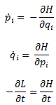
Hamilton's Canonical Equations of motion:-

• Co-ordinates cyclic in Lagrangian will also be cyclic in Hamiltonian.
• Canonical transformations are characterized by the property that they leave the form of Hamilton's equations of motion invarient.
• Lagrange's equation of motion are covarient w.r.t. point transformations (Q_j=Q_j(q_j,t) and if we define P_j as,
  

         

     

           the Hamilton's canonical equation will also be covarient.

• Consider the transformations
  
         Q_j=Q_j(p,q,t)
         P_j=P_j(p,q,t)
         where Q_j and P_j are new set of co-ordinates.
• For Q_j and P_j to be canonical they should be able to be expressed in Hamiltonian form of equations of motion i.e.,
  
  
  
  
  
  
  
  
  
  
  
  
  
  
  
  
  
  
   where,  K=K(Q,P,t) and is substitute of Hamiltonian H of old set in new set of co-ordinates.
• Q_j and P_j to be canonical must also satisfy modified Hamilton's principle i.e.,
  
  
  
  
  
  
  
  
  
  
  
  
  
  
• Using same principle for old set q_j and p_j
  
                             (1)
  
  
   where F is any function of phase space co-ordinates with continous second derivative.
• Term ∂F/∂t in 1 contributes to the variation of the action integral only at end points and will therefore vanish if F is a function of (q,p,t) or (Q,P,t) or any mixture of phase space co-ordinates since they have zero variation at end points.
  
• F is useful for specifying the exact form of anonical transformations only when half of the variables (except time) are from the old set and half from the new set.
  
• F acts as bridge between two sets of canonical variables and is known as generating function of transformations.
  

In next post I'll discuss more about generating functions , lagrange and poisson brackett.

Constrains and constrained motion

• A constrained motion is a motion which can not proceed arbitrary in any manner.
• Particle motion can be restricted to occur (1) along some specified path (2) on surface (plane or curved) arbitrarily oriented in space.
• Imposing constraints on a mechanical system is done to simplify the mathematical description of the system.
• Constraints expressed in the form of equation f(x₁,y₁,z₁,......,x_n,y_n,z_n :t)=0 are called holonomic constraints.
• Constraints not expressed in this fashion are called non-holonomic constraints.
• Scleronomic conatraints are independent of time.
• Constraints containing time explicitely are called rehonomic.
• Therefore a constraint is either

          "Scleronomic where constraints relations does not depend on time or rheonomic where constraints relations depends explicitly on time "
          and either
           "holonomic where constraints relations can be made independent of velocity or non-holonomic where these relations are irreducible functions of velocity"

Constraints types of some physicsl systems are given below in the table

Wave velocity in a continuous system

• Any system whose particle motion are governed by classical wave equation is a system in which harmonic waves of any wavelength can travel with the speed v
  
  
• The value of v depends on the elastic and inertial properties of the system under consideration.
  

(1) Transverse wave on a stretched string

• Displacement of the string is governed by the equation
  
  
  
  
  
  
  Where T is the tension and µ is the linear density (mass per unit length of the string)
  
• Velocity of wave on the string is
  v=√(T/μ)
  v is the velocity of the wave.
  
• Medium through which waves travel will offer impedance to these waves.
  
• If the medium is loss less i.e., it does not have any resistive or dissipative components, the impedance is solely determined by its inertia and elasticity.
  
• Characteristic impedance of string is determined by
  Z=T/v=√(μT)=μv
  
• Since v is determined by the inertia and elasticity this shows that impedance is also governed by these two properties of the medium.
  
• For loss-less medium impedance is real quantity and it is complex if the medium is dissipative.
  

(2) Longitudinal waves in uniform rod

• Equation for longitudinal vibrations of a uniform rod is
  
  
  
  
  
  
  
• where ξ (x,t )→displacement
  Y is young’s modulus of the rod
  ρ is the density
  
• Velocity of longitudinal wave in rod is
  v=√(Y/ρ)
  

(3) Electromagnetic waves in space

• When electric and magnetic field vary in time they produce EM waves.
  
• An oscillating charge has an oscillating electric and magnetic fields around it and hence produces EM waves.
  
• Example: - (1) Electrons falling from higher to lower energy orbit radiates EM waves of particular wavelength and frequency. (2) The motion of electrons in an antenna radiates EM waves by a process called Bramstrhlung.
  
• Propagation of EM waves in a medium is also due to inertial and elastic properties of the medium.
  
• Every medium (including vacuum) has inductive properties described by magnetic permeability µ of the medium.
  
• This property provides magnetic inertia of the medium.
  
• Elasticity of the medium is provided by the capacitive property called electrical permittivity ε of the medium.
  
• Permeability µ stores magnetic energy and the permittivity ε stores the electric field energy.
  
• This EM energy propagates in the medium in the form of EM waves.
  
• Electric and magnetic fields are connected by Maxwell’s Equations (dielectric medium)
  ∇×H =ε (∂E )/∂t
  ∇×E = - μ (∂H⃗)/∂t
  ε(∇∙E⃗)=ρ
  ∇∙H =0
  
• Here in above equations E ⃗ is electric field , H ⃗ is the magnetic field and ρ is charge density
  

SYLLABUS FOR PHYSICAL SCIENCES PAPER I AND PAPER II

The full Syllabus for Part B of Paper I and Part B of Paper II.

The syllabus for Part A of Paper II comprises Sections I-VI.

I. Mathematical Methods of Physics

Dimensional analysis; Vector algebra and vector calculus; Linear algebra, matrices, Cayley Hamilton theorem, eigenvalue problems; Linear differential equations; Special functions (Hermite, Bessel, Laguerre and Legendre); Fourier series, Fourier and Laplace transforms; Elements of complex analysis: Laurent series-poles, residues and evaluation of integrals; Elementary ideas about tensors; Introductory group theory, SU(2), O(3); Elements of computational techniques: roots of functions, interpolation, extrapolation, integration by trapezoid and Simpson’s rule, solution of first order differential equations using Runge-Kutta method; Finite difference methods; Elementary probability theory, random variables, binomial, Poisson and normal distributions.

II. Classical Mechanics

Newton’s laws; Phase space dynamics, stability analysis; Central-force motion; Two-body collisions, scattering in laboratory and centre-of-mass frames; Rigid body dynamics, moment of inertia tensor, non-inertial frames and pseudoforces; Variational principle, Lagrangian and Hamiltonian formalisms and equations of motion; Poisson brackets and canonical transformations; Symmetry, invariance and conservation laws, cyclic coordinates; Periodic motion, small oscillations and normal modes; Special theory of relativity, Lorentz transformations, relativistic kinematics and mass–energy equivalence.

III. Electromagnetic Theory

Electrostatics: Gauss’ Law and its applications; Laplace and Poisson equations, boundary value problems; Magnetostatics: Biot-Savart law, Ampere's theorem, electromagnetic induction; Maxwell's equations in free space and linear isotropic media; boundary conditions on fields at interfaces; Scalar and vector potentials; Gauge invariance; Electromagnetic waves in free space, dielectrics, and conductors; Reflection and refraction, polarization, Fresnel’s Law, interference, coherence, and diffraction; Dispersion relations in plasma; Lorentz invariance of Maxwell’s equations; Transmission lines and wave guides; Dynamics of charged particles in static and uniform electromagnetic fields; Radiation from moving charges, dipoles and retarded potentials.

IV. Quantum Mechanics

Wave-particle duality; Wave functions in coordinate and momentum representations; Commutators and Heisenberg's uncertainty principle; Matrix representation; Dirac’s bra and ket notation; Schroedinger equation (time-dependent and time-independent); Eigenvalue problems such as particle-in-a-box, harmonic oscillator, etc.; Tunneling through a barrier; Motion in a central potential; Orbital angular momentum, Angular momentum algebra, spin; Addition of angular momenta; Hydrogen atom, spin-orbit coupling, fine structure; Time-independent perturbation theory and applications; Variational method; WKB approximation;

Time dependent perturbation theory and Fermi's Golden Rule; Selection rules; Semi-classical theory of radiation; Elementary theory of scattering, phase shifts, partial waves, Born approximation; Identical particles, Pauli's exclusion principle, spin-statistics connection; Relativistic quantum mechanics: Klein Gordon and Dirac equations.

V. Thermodynamic and Statistical Physics

Laws of thermodynamics and their consequences; Thermodynamic potentials, Maxwell relations; Chemical potential, phase equilibria; Phase space, micro- and macrostates; Microcanonical, canonical and grand-canonical ensembles and partition functions; Free Energy and connection with thermodynamic quantities; First- and second-order phase transitions; Classical and quantum statistics, ideal Fermi and Bose gases; Principle of detailed balance; Blackbody radiation and Planck's distribution law; Bose-Einstein condensation; Random walk and Brownian motion; Introduction to nonequilibrium processes; Diffusion equation.

VI. Electronics

Semiconductor device physics, including diodes, junctions, transistors, field effect devices, homo and heterojunction devices, device structure, device characteristics, frequency dependence and applications; Optoelectronic devices, including solar cells, photodetectors, and LEDs; High-frequency devices, including generators and detectors; Operational amplifiers and their applications; Digital techniques and applications (registers, counters, comparators and similar circuits); A/D and D/A converters; Microprocessor and microcontroller basics.

VII. Experimental Techniques and data analysis

Data interpretation and analysis; Precision and accuracy, error analysis, propagation of errors, least squares fitting, linear and nonlinear curve fitting, chi-square test; Transducers (temperature, pressure/vacuum, magnetic field, vibration, optical, and particle detectors), measurement and control; Signal conditioning and recovery, impedance matching, amplification (Op-amp based, instrumentation amp, feedback), filtering and noise reduction, shielding and grounding; Fourier transforms; lock-in detector, box-car integrator, modulation techniques.

Applications of the above experimental and analytical techniques to typical undergraduate and graduate level laboratory experiments.

VIII. Atomic & Molecular Physics

Quantum states of an electron in an atom; Electron spin; Stern-Gerlach experiment; Spectrum of Hydrogen, helium and alkali atoms; Relativistic corrections for energy levels of hydrogen; Hyperfine structure and isotopic shift; width of spectral lines; LS & JJ coupling; Zeeman, Paschen Back & Stark effect; X-ray spectroscopy; Electron spin resonance, Nuclear magnetic resonance, chemical shift; Rotational, vibrational, electronic, and Raman spectra of diatomic molecules; Frank – Condon principle and selection rules; Spontaneous and stimulated emission, Einstein A & B coefficients; Lasers, optical pumping, population inversion, rate equation; Modes of resonators and coherence length.

IX. Condensed Matter Physics

Bravais lattices; Reciprocal lattice, diffraction and the structure factor; Bonding of solids; Elastic properties, phonons, lattice specific heat; Free electron theory and electronic specific heat; Response and relaxation phenomena; Drude model of electrical and thermal

conductivity; Hall effect and thermoelectric power; Diamagnetism, paramagnetism, and ferromagnetism; Electron motion in a periodic potential, band theory of metals, insulators and semiconductors; Superconductivity, type – I and type - II superconductors, Josephson junctions; Defects and dislocations; Ordered phases of matter, translational and orientational order, kinds of liquid crystalline order; Conducting polymers; Quasicrystals.

X. Nuclear and Particle Physics

Basic nuclear properties: size, shape, charge distribution, spin and parity; Binding energy, semi-empirical mass formula; Liquid drop model; Fission and fusion; Nature of the nuclear force, form of nucleon-nucleon potential; Charge-independence and charge-symmetry of nuclear forces; Isospin; Deuteron problem; Evidence of shell structure, single- particle shell model, its validity and limitations; Rotational spectra; Elementary ideas of alpha, beta and gamma decays and their selection rules; Nuclear reactions, reaction mechanisms, compound nuclei and direct reactions; Classification of fundamental forces; Elementary particles (quarks, baryons, mesons, leptons); Spin and parity assignments, isospin, strangeness; Gell-Mann-Nishijima formula; C, P, and T invariance and applications of symmetry arguments to particle reactions, parity non-conservation in weak interaction; Relativistic kinematics.

Learn Physics through physics notes and study material: 5 Secrets to Cracking Competitive Exams

Visit this post to learn more
Learn Physics through physics notes and study material: 5 Secrets to Cracking Competitive Exams: "They’re not the kind of exams you’re used to in school, but you know you have to prepare hard for them if you want to go to college. Almost ..."

Waves in continous medium

• There are essentially two ways of transporting energy from one place to another (a) Actual transport of matter for example a fired bullet and (b) Waves carry energy but there is no transport of matter for example sound waves carry energy so thay can move diphagram of the ear.
• Here we will consider the oscillations of open or unbounded systems i.e., systems having no outer boundaries.
• If such system is disturbed , waves travel in the system with a speed determined by the properties of the system.
• Waves are not reflected back in such a system.
• The waves generated by driving force are called travelling waves ; these waves travel from the point where the driving force produces the disturbance.
• If the driving force produces a harmonic disturbance the travelling wave it produces are called harmonic travelling waves.
• In the steady state, all moving parts of the system oscillates with simple harmonic motion at the driving frequency.
• Waves where the displacements or oscillations are transverse (i.e., perpandicular) to the direction of wave propagation is called transverse wave.
• The wavelength (denoted by λ) of the wave is defined as the distance, measured along the direction of the propagation of the wave, between two nearest points which are in the same state of viberation.
• Wavelength λ is just the distance travelled by the wave during one time period T of particle oscillation. Thus wave velocity
  v=λ/T=λν
  where ν=1/T - is the frequency of the wave.
• This relation between wave velocity, frequency and wavelength also holds for longitudinal waves in which the displacements or oscillation in the medium are parallel to the direction of wave propagation.
• Waves in spring and sound waves are longitudinal waves.
• Wavelength for longitudinal waves is the distance between two successive compressions or rarefactions.
• Sound waves are also compressional.
• Assumptions that are made while obtaining wave equation are:-
  1. Amplitude A of particle oscillations does not change in course of the propagation of wave.
  2. The medium is isotopic and homogeneous so that velocity of wave does not chance from place to  place
• Displacement of particle at x at any time t is
  Ψ(x,t) = A sin{2π(t-x/v)/T)}
• The function Ψ(x,t) repeats itself in a distance λ . Wavelength of a wave is also known as spatial periodicity of the wave.
• The wave is thus doubly periodic. It has temporal periodicity T and spatial periodicity λ.
• Let us define quantities
  k=2π/λ and
  ω=2π/T
  then wave function can be written as
  Ψ(x,t) = A sin{ωt-kx}
  where quantity k is known as wave number of the wave and ω is called angular frequency of particle oscillations in wave.
• Harmonic wave travelling in
  + x direction    :     Ψ(x,t) = A sin{ωt-kx}
  - x direction    :     Ψ(x,t) = A sin{ωt+kx}
  above equations can also be equally well described by cosine function.
• Classicsl wave equation is
  
  
  
  
  

• Important inferences from above wave equation
  1. Whenever second order time derivative of any physical quantity is related to second order space derivative as in above equation , a wave of some sort must travell in the medium.
  2. Velocity of that wave is given by the square root of the coefficent of second order space derivative.
• Individual derivatives which makes up the medium do not propagate through the medium with the wave; they merely oscillates ( transversly or longitudinally) about there equilibrium positions.
• It is their phase relationship which we observe as wave.
• Wave velocity is also called phase velocity with which crest or troughs in case of transverse wave and compressions or rarefactions in case of longitudinal waves travell through the medium.
• The phase velocity is given by
  v=λ/T=λν
  or,
  v=ω/k
• Ψ(x,t)=f(vt-x) is the solution of the above given wave equation.

Uncertainity Principle

Uncertainity principle says that "If a measurement of position is made with accuracy Δx and if the measurement of momentum is made simultaneously with accuracy Δp , then the product of two errors can never be smaller than a number of order h
ΔpΔx≥(∼h)                                  (1)
Similarly if the energy of the syatem is measured to accuracy ΔE , then time to which this measurement refers must have a minimum uncertainity given by
ΔEΔt≥(∼h)                                    (2)
In generalised sence we can say that if  Δq is the error in the measurement of any co-ordinate and Δp is the error in its canonically conjugate momentum then we have,
ΔpΔq≥(∼h)                                  (3)
Consider the relation between the range of position Δx and range of wave number Δk appearing in a wave packet then
ΔxΔk≥1                                                     (4)
and this is a general property not restricted to quantum mechanics. Uncertainity principle is obtaines when the following quantum mechanical interpretation of quantities appearing in above equation are taken into account.
(1) The de-Brogli equation p=hk creates a relationship between wave number and momentum , which is not present in classical mechanics.
(2) Whenever either the momentum or the position of an electron is measured , the result is always some definite number. A classical wave packet always covers a range of positions and range of wave numbers.
Δx is a measure of minimum uncertainity or lack of complete determination of the position that can be ascribed to the electron. and Δk is the measure of minimum uncertainity or lack of complete determination of the momentum that can be ascribed to it.

Relation of spreading wave packet to uncertainity principle
Narrower the wave packet to begin with , the more rapidly it spreads. Because of the confinement of the packet within the region Δx₀ the fourier analysis contains many waves of length of order of Δx₀ , hence momenta p≅h/Δx₀
therefore
Δv≅p/m≅h/mΔx₀
Although average velocity of the packet is equal to the group velocity , there is still a strong chance that the actual velocity will fluctuate about this average by the same amount. The distance covered by the particle is not completely determined but it may vary as much as
Δx≅tΔv≅ht/mΔx₀
The spread of the wave packet may therefore be regarded as one of the manifestations of the lack of complete determination of initial velocity necesarily associated with the narrow wave packet.

Relation of stability of atom to uncertainity principle
From uncertainity principle if an electron is localized it must have on an average a high momentum and have high kinetic energy as it takes energy to localize a particle. According to uncertainity principle it takes a momentum  Δp≅h/Δx and an energy nearly equal to h²/2m(Δx)² to keep an electron localised within a region Δx. Momentum creates a pressure which tends to oppose localization of the electron. In an atom the pressure is opposed by the force attracting the electron back to the nucleus. Thus the electron will come to equilibrium when the attractive forces balances the effective pressure and, this way , the mean radius of the lowest quantum state is determined. This point of balance can be found from the condition that total energy must be minimum. Thus we have
W≅  (h²/2m(Δx)²) - (e²/Δx)
Differentiating both the sides w.r.t. Δx and making ∂W/∂(Δx) = 0 we get
Δx≅h²/me²
THis result is just the radius of first Bohr orbit although not exact but qualitative.. The limitation of the localizability of the electron is inherent in the wave-particle nature of matter. In order to have an electron in very small space , we must have very high fourier components in its wave function and therefore the possibility of very high moments. There is no way to force an electron to occpy a well defined position and still remain at rest.

Force on a conductor

We have already learned in our previous discussion that field inside a conductor is zero and the field immidiately outside is
E_n=n(σ/ε₀)                               (1)
where n is the unit normal vector to the surface of the conductor. We also know that any charge a conductor may carry is distributed on the surface of the conductor.
In presence of an electric field this surface charge will experience a force. If we consider a small area element ΔS of the surface of the conductor then force acting on area element is given by
ΔF=(σΔS).E₀       (2)
where σ is the surface charge density of the conductor , (σΔS) is the amount of charge on the area element ΔS and E₀ is the field in the region where charge element (σΔS) is located.
Now there are two fields present  E_σ and E₀ and the resultant field both inside and outside the conductor near area element  ΔS would be equal to the superposition of both the fields  E_σ and E₀ . Figure below shows the directions of both the fields inside and outside the conductor

Now field E₀ has same value both inside and outside the conductor and surface element ΔS suffers discontinuty because of the charge on the surface and this makes field  E_σ on either side pointing away from the surfaceas shown in the figure given above. Since E=0 inside the conductor

E<sub>in=E₀+E_σ=0
E_in=E₀=E_σ
Since direction of  E_σ and E₀ are opposite to each other and outside the conductor near its surface
E_out=E₀+E_σ=2E₀
Thus , E₀ =E/2                      (3)
Equation (2) thus becomes,regardless of the of ΔF=½(σΔS).E                  (4)
From equation 4 , force acting per unit area of the surface of the conductor is
f=½σ.E                                       (5)
Here  is the  E_σ electric field intensity created by charge on area element ΔS at the point very close to this area element. In this region this area element behaves as infinite uniformly charged sheet hence we have,
E_σ=σ/2ε₀                                                  (6)
Now,
E=2E₀=2E_σ=(σ/ε₀)n=E_n
which is in accordance with equation 1. Hence from equation 5
f=σ²/2ε₀ = (ε₀E²/2)n                (7)
This quantity f is known as surface density of force. From equation 7 we can conclude that regardless of the sign of σ and hence direction of E , f is always directed in outward direction of the conductor.

Electric field due to charged conductor

In our previous post we have discussed that electric field inside a conductor is zero and any charge the conductor may carry shall be distributed on the surface of the conductor. For our discussion consider a conductor carrying charge on its surface again consider a small surface element ds over which we can consider surface charge density σ to be approximately constant.
For positive charge distributed over the surface of the conductor , electric field E would be directed at right angels to the surface pointing in outwards direction. Now E due to charge carrying conductor can be calculated using Gauss's law. For this draw a Gaussin cylendrical surface as shown below in the figure

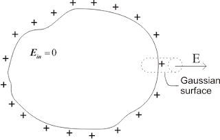
Now S is the area of cross-section of the surface. The flux due to cylendrical surface is zero because electric field and the normal to the surface are perpandicular to each other. Since electric field inside the conductor is zero hence only contribution to the flux is due to the chare on area S lying outside the  surface of the conductor. So total flux through the surface would be

From Gauss's law,
ES=q/ε₀=σS/ε₀
or,
E=σ/ε₀
and this is the required relation for the field of charged conductor

How conductors behave in the presence of electrostatic field

We know that conductors like copper , silver, aluminium etc. , have very large number of free and movable charge carriers , usually one free electron per atom. These free electrons are not bound to its atom and moves freely in the space between the atoms. These free electrons can move under the action of electric field present inside the conductor.
Consider an arbitrary shaped conductor placed inside an electric field such that the field in the conductor is directed from left to right. As a result of this electric field positive charge in the conductor moves from left to right and negative charge moves from right to left. As a result there is a surplus negative charge on the left side of the conductor and a surplus positive charge on the right side of the conductor. This induced surplus chare on both the sides of the conductor acts as a source of an induced electric field which is directed from right to left i.e., in the direction opposite to the initial electric field.
Now with the increase in the amount of induced electric charges, magnitude of induced electric field also increases which cancels out the original electric field having direction opposite to it. This results in a progressive decrease in total field inside the conductor. In the end induced electric field cancels out all the initial electric field thus reaching an electrostatic equilibrium where there is zero electric field at each and every point inside the conductor. Hence we can conclude thet,
E=0 inside the conductor
Now if we apply Gauss's law to any arbitrary surface inside the conductor then total charge enclosed by the gaussian surface equals zero as vector E=0 at all points inside the gaussian surface. From this we conclude that
Al the excess charge (if any) is distributed on the surface of the conductor
We have established the fact that there is no E inside the conductor so tangential component of E is zero on the surface of the conductor hence the potential difference between any two points on the surface of the conductor would also be zero. This indicates that the surface of conductor in electrostatics is equipotential one. Since there is no E inside the conductor so all the points in the conductor are at the same potential.
This is almost all I intended to write in this topic however if you have any doubts then let me know and also you can tell me about the topic you want me to write next in the blog.

Vector Differentiation 2

In this post we'll discuss about Divergence and curl of vector fields.
Divergence of vector fields
We already know about dot product of two vectors. Now consider a vector field φ(x,y,z) and we now find out the dot product of operator ∇ and vector field φ(x,y,z). So,




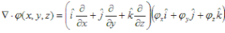
or,






Thus we see that dot product of del operator with a vector field is a scalar quantity. This scalar quantity ∇⋅φ(x,y,z) is known as divergence of the vector function φ(x,y,z). Thus,
∇⋅φ = div φ='divergence of φ'
Physically we can say that divergence of any vector field is the measure of how much the vector diverges (spreads out) or converges at a given point. Divergence of a vector at any point can be positive, negative and zero illustrated below in the figures.








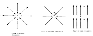
Consider the example of a fluid, if the Divergence is positive at any point in a fluid , then either the fluid is expanding and its density at the point is falling with time or the point is a source of the fluid. Again if the divergence is negative , then either the fluid is contracting and the density is rising at the point or the point is at the sink. If the flux entering field space is equal to that leaving it then divergence of the field is zero i.e. there is no source or sink and its density is also not changing which means that liquid is incompressible. Any vector having its divergence equal to zero is known as solenoidal vector.
Curl of the vector fields
We have already discussed the dot product of del operator (∇) with a vector which is known as divergence of vector. Now let us find the cross product of operator ∇ with the vector field φ(x,y,z). Thus,






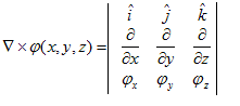
or






Thus we have seen that curl of a vector function is a vector whose components can be written by usual rule of cross products. Any vector field φ(x,y,z) for which ∇xφ(x,y,z) = 0 is said to be irrotational.The curl of a scalar field makes no sense.The curl of a vector field φ(x,y,z) at a point P may be regarded as a measure of the circulation or how much the field curls around a point.
In our next discussion we'll learn about second derivatives of vector fields and we'll discuss more about divergence and curl while discussing vector integral calculas.